如果你也在 怎样代写有限元方法finite differences method 这个学科遇到相关的难题，请随时右上角联系我们的24/7代写客服。有限元方法finite differences method在数值分析中，是一类通过用有限差分逼近导数解决微分方程的数值技术。空间域和时间间隔（如果适用）都被离散化，或被分成有限的步骤，通过解决包含有限差分和附近点的数值的代数方程来逼近这些离散点的解的数值。

有限元方法finite differences method有限差分法将可能是非线性的常微分方程（ODE）或偏微分方程（PDE）转换成可以用矩阵代数技术解决的线性方程系统。现代计算机可以有效地进行这些线性代数计算，再加上其相对容易实现，使得FDM在现代数值分析中得到了广泛的应用。今天，FDM与有限元方法一样，是数值解决PDE的最常用方法之一。

couryes-lab™ 为您的留学生涯保驾护航 在代写有限元方法Finite Element Method方面已经树立了自己的口碑, 保证靠谱, 高质且原创的统计Statistics代写服务。我们的专家在代写有限元方法Finite Element Method代写方面经验极为丰富，各种代写有限元方法Finite Element Method相关的作业也就用不着说。

数学代写|有限元方法代写Finite Element Method代考|Reduced Integration Element (RIE)

When equal interpolation of $w_h^e(x)$ and $\phi_x^e(x)$ is used $(m=n)$, all sub-matrices in Eq. (5.3.15) are of the same order: $n \times n$, where $n$ is the number of terms in the polynomial (or $n-1$ is the degree of interpolation). The element coefficient matrices $K_{i j}^{11}, K_{i j}^{12}$ as well as the first part of $K_{i j}^{22}$ are evaluated exactly. The second part of $K_{i j}^{22}$ is to be evaluated using reduced integration. For the choice of linear interpolation functions, and for element-wise constant values of $G_e A_e K_s$ and $E_e I_e$, the matrices in Eq. (5.3.15) for this case have the following explicit values (when $k_f^e=0$ ):
$$
\begin{gathered}
\mathbf{K}^{11}=\frac{G_e A_e K_s}{h_e}\left[\begin{array}{rr}
1 & -1 \
-1 & 1
\end{array}\right], \quad \mathbf{K}^{12}=\frac{G_e A_e K_s}{2}\left[\begin{array}{rr}
-1 & -1 \
1 & 1
\end{array}\right] \
\mathbf{K}^{22}=\frac{E_e I_e}{h_e}\left[\begin{array}{rr}
1 & -1 \
-1 & 1
\end{array}\right]+\frac{G_e A_e K_s h_e}{4}\left[\begin{array}{lr}
1 & 1 \
1 & 1
\end{array}\right]
\end{gathered}
$$
where one-point integration is used to evaluate the second part of $\mathbf{K}^{22}$. Note that $\mathbf{K}^{11}, \mathbf{K}^{12}$, and the first part of $\mathbf{K}^{22}$ can be evaluated exactly with onepoint quadrature (i.e., numerical integration) when $E_e I_e$ and $G_e A_e K_s$ are constant because the integrands of these coefficients are constant. Hence, one-point integration for $\mathbf{K}^{\alpha \beta}$ satisfies all requirements. The resulting beam element is termed the reduced integration element (RIE). Expressing Eq. (5.3.15), with $\mathbf{K}^{\alpha \beta}$ from Eq. (5.3.25a), and rearranging the nodal vector, we obtain
$$
\frac{G_e A_e K_s}{4 h_e}\left[\begin{array}{cccc}
4 & -2 h_e & -4 & -2 h_e \
-2 h_e & h_e^2\left(1+4 \mu_e\right) & 2 h_e & h_e^2\left(1-4 \mu_e\right) \
-4 & 2 h_e & 4 & 2 h_e \
-2 h_e & h_e^2\left(1-4 \mu_e\right) & 2 h_e & h_e^2\left(1+4 \mu_e\right)
\end{array}\right]\left{\begin{array}{c}
w w_1^e \
S_1^e \
w_2^e \
s_2^e
\end{array}\right}=\left{\begin{array}{c}
q_1^e \
0 \
q_2^e \
0
\end{array}\right}+\left{\begin{array}{c}
Q_1^e \
Q_2^{\prime} \
Q_3^{\prime} \
Q_4^{\prime}
\end{array}\right}
$$
where
$$
\mu_e=E_e I_e / G_e A_e K_s h_e^2
$$
To resemble Eq. (5.3.24), we can write the element equations of the RIE element as
$$
\begin{gathered}
\frac{E_e I_e}{6 \mu_e h_e^3}\left[\begin{array}{cccc}
6 & -3 h_e & -6 & -3 h_e \
-3 h_e & h_e^2\left(1.5+6 \mu_e\right) & 3 h_e & h_e^2\left(1.5-6 \mu_e\right) \
-6 & 3 h_e & 6 & 3 h_e \
-3 h_e & h_e^2\left(1.5-6 \mu_e\right) & 3 h_e & h_e^2\left(1.5+6 \mu_e\right)
\end{array}\right]\left{\begin{array}{c}
w_1^e \
s_l^e \
w_2 \
s_2^*
\end{array}\right}=\left{\begin{array}{c}
q_1^e \
0 \
q_2^e \
0
\end{array}\right}+\left{\begin{array}{c}
Q_1^e \
Q_2^e \
Q_3^2 \
Q_4^3
\end{array}\right} \
q_i^e=\int_0^{h_e} \psi_i^e q_e d \bar{x},(i=1,2)\left(\psi_i^e\right. \text { are linear) } \
\mu_e=\frac{E_e I_e}{G_e A_e K_s h_e^2}
\end{gathered}
$$

数学代写|有限元方法代写Finite Element Method代考|Governing Equations

In this section, the finite element model of axisymmetric bending of circular plates using the classical plate theory (i.e., the theory in which transverse shear strain is assumed to be zero) is developed. We select the cylindrical coordinate system $(r, \theta, z)$ such that $r$ is the radial coordinate outward from the center of the plate $(0 \leq r \leq R), z$ denotes the transverse coordinate $(-H / 2 \leq$ $z \leq H / 2$ ), where $H$ is the total thickness of the plate, and $\theta$ is the angular coordinate ( $0 \leq \theta \leq 2 \pi)$, as shown in Fig. 5.4.1.

Governing equations of circular plates subjected to loads as well as boundary conditions that are independent of the angular coordinate $\theta$ can be formulated in terms of the radial coordinate $r$ alone. Thus, the axisymmetric bending of circular plates is a one-dimensional problem, as discussed next (see Fig. 5.4.2).

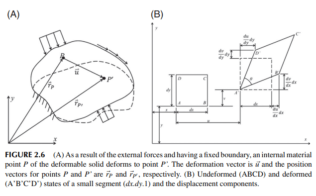
The total displacements $\left(u_r, u_\theta, u_z\right)$ along the three coordinate directions $(r, \theta, z)$, as implied by the Love-Kirchhoff hypothesis for plates, which is the same as the Euler-Bernoulli hypothesis for beams, are given by
$$
u_r(r, z)=-z \frac{d w}{d r}, u_\theta(r, z)=0, u_z(r, z)=w(r)
$$
where $w$ denotes the transverse displacement of a point on the midplane of the plate. The nonzero linear strain components referred to the cylindrical coordinate system are given by (see Reddy [1, 2] and Ugural [6])
$$
\varepsilon_{r r}=\frac{d u_r}{d r}=-z \frac{d^2 w}{d r^2}, \varepsilon_{\theta \theta}=\frac{u_r}{r}=-\frac{z}{r} \frac{d w}{d r}
$$

有限元方法代考

数学代写|有限元方法代写Finite Element Method代考|Reduced Integration Element (RIE)

当使用$w_h^e(x)$和$\phi_x^e(x)$的相等插值$(m=n)$时，Eq.(5.3.15)中的所有子矩阵都是相同的顺序:$n \times n$，其中$n$是多项式中的项数(或$n-1$是插值的程度)。对元素系数矩阵$K_{i j}^{11}, K_{i j}^{12}$和$K_{i j}^{22}$的第一部分进行了精确的求值。$K_{i j}^{22}$的第二部分将使用简化的集成进行评估。对于线性插值函数的选择，对于$G_e A_e K_s$和$E_e I_e$的逐元常数值，在这种情况下，式(5.3.15)中的矩阵具有以下显式值(当$k_f^e=0$时):
$$
\begin{gathered}
\mathbf{K}^{11}=\frac{G_e A_e K_s}{h_e}\left[\begin{array}{rr}
1 & -1 \
-1 & 1
\end{array}\right], \quad \mathbf{K}^{12}=\frac{G_e A_e K_s}{2}\left[\begin{array}{rr}
-1 & -1 \
1 & 1
\end{array}\right] \
\mathbf{K}^{22}=\frac{E_e I_e}{h_e}\left[\begin{array}{rr}
1 & -1 \
-1 & 1
\end{array}\right]+\frac{G_e A_e K_s h_e}{4}\left[\begin{array}{lr}
1 & 1 \
1 & 1
\end{array}\right]
\end{gathered}
$$
其中一点积分用于计算$\mathbf{K}^{22}$的第二部分。请注意，当$E_e I_e$和$G_e A_e K_s$为常数时，$\mathbf{K}^{11}, \mathbf{K}^{12}$和$\mathbf{K}^{22}$的第一部分可以用一点正交(即数值积分)精确地求值，因为这些系数的积分是常数。因此，$\mathbf{K}^{\alpha \beta}$的一点集成满足所有需求。得到的梁单元称为简化积分单元(RIE)。用Eq.(5.3.15)中的$\mathbf{K}^{\alpha \beta}$表示Eq. (5.3.25a)，重新排列节点向量，得到
$$
\frac{G_e A_e K_s}{4 h_e}\left[\begin{array}{cccc}
4 & -2 h_e & -4 & -2 h_e \
-2 h_e & h_e^2\left(1+4 \mu_e\right) & 2 h_e & h_e^2\left(1-4 \mu_e\right) \
-4 & 2 h_e & 4 & 2 h_e \
-2 h_e & h_e^2\left(1-4 \mu_e\right) & 2 h_e & h_e^2\left(1+4 \mu_e\right)
\end{array}\right]\left{\begin{array}{c}
w w_1^e \
S_1^e \
w_2^e \
s_2^e
\end{array}\right}=\left{\begin{array}{c}
q_1^e \
0 \
q_2^e \
0
\end{array}\right}+\left{\begin{array}{c}
Q_1^e \
Q_2^{\prime} \
Q_3^{\prime} \
Q_4^{\prime}
\end{array}\right}
$$
在哪里
$$
\mu_e=E_e I_e / G_e A_e K_s h_e^2
$$
与式(5.3.24)相似，我们可以将RIE单元的元素方程写成
$$
\begin{gathered}
\frac{E_e I_e}{6 \mu_e h_e^3}\left[\begin{array}{cccc}
6 & -3 h_e & -6 & -3 h_e \
-3 h_e & h_e^2\left(1.5+6 \mu_e\right) & 3 h_e & h_e^2\left(1.5-6 \mu_e\right) \
-6 & 3 h_e & 6 & 3 h_e \
-3 h_e & h_e^2\left(1.5-6 \mu_e\right) & 3 h_e & h_e^2\left(1.5+6 \mu_e\right)
\end{array}\right]\left{\begin{array}{c}
w_1^e \
s_l^e \
w_2 \
s_2^*
\end{array}\right}=\left{\begin{array}{c}
q_1^e \
0 \
q_2^e \
0
\end{array}\right}+\left{\begin{array}{c}
Q_1^e \
Q_2^e \
Q_3^2 \
Q_4^3
\end{array}\right} \
q_i^e=\int_0^{h_e} \psi_i^e q_e d \bar{x},(i=1,2)\left(\psi_i^e\right. \text { are linear) } \
\mu_e=\frac{E_e I_e}{G_e A_e K_s h_e^2}
\end{gathered}
$$

数学代写|有限元方法代写Finite Element Method代考|Governing Equations

本节采用经典板理论(即假定横向剪切应变为零的理论)建立了圆板轴对称弯曲的有限元模型。我们选择柱坐标系$(r, \theta, z)$，其中$r$为板中心向外的径向坐标$(0 \leq r \leq R), z$为横向坐标$(-H / 2 \leq$$z \leq H / 2$)，其中$H$为板的总厚度，$\theta$为角坐标($0 \leq \theta \leq 2 \pi)$，如图5.4.1所示)。

受载荷作用的圆形板的控制方程以及与角坐标$\theta$无关的边界条件可以单独用径向坐标$r$表示。因此，圆板的轴对称弯曲是一个一维问题，如下面的讨论(见图5.4.2)。

板的Love-Kirchhoff假设(与梁的Euler-Bernoulli假设相同)所隐含的沿三个坐标方向$(r, \theta, z)$的总位移$\left(u_r, u_\theta, u_z\right)$由式给出
$$
u_r(r, z)=-z \frac{d w}{d r}, u_\theta(r, z)=0, u_z(r, z)=w(r)
$$
式中$w$表示板中部某点的横向位移。圆柱坐标系下的非零线性应变分量由(见Reddy[1,2]和Ugural[6])给出。
$$
\varepsilon_{r r}=\frac{d u_r}{d r}=-z \frac{d^2 w}{d r^2}, \varepsilon_{\theta \theta}=\frac{u_r}{r}=-\frac{z}{r} \frac{d w}{d r}
$$

统计代写请认准statistics-lab™. statistics-lab™为您的留学生涯保驾护航。

金融工程代写

金融工程是使用数学技术来解决金融问题。金融工程使用计算机科学、统计学、经济学和应用数学领域的工具和知识来解决当前的金融问题，以及设计新的和创新的金融产品。

非参数统计代写

非参数统计指的是一种统计方法，其中不假设数据来自于由少数参数决定的规定模型；这种模型的例子包括正态分布模型和线性回归模型。

广义线性模型代考

广义线性模型（GLM）归属统计学领域，是一种应用灵活的线性回归模型。该模型允许因变量的偏差分布有除了正态分布之外的其它分布。

术语 广义线性模型（GLM）通常是指给定连续和/或分类预测因素的连续响应变量的常规线性回归模型。它包括多元线性回归，以及方差分析和方差分析（仅含固定效应）。

有限元方法代写

有限元方法（FEM）是一种流行的方法，用于数值解决工程和数学建模中出现的微分方程。典型的问题领域包括结构分析、传热、流体流动、质量运输和电磁势等传统领域。

有限元是一种通用的数值方法，用于解决两个或三个空间变量的偏微分方程（即一些边界值问题）。为了解决一个问题，有限元将一个大系统细分为更小、更简单的部分，称为有限元。这是通过在空间维度上的特定空间离散化来实现的，它是通过构建对象的网格来实现的：用于求解的数值域，它有有限数量的点。边界值问题的有限元方法表述最终导致一个代数方程组。该方法在域上对未知函数进行逼近。[1] 然后将模拟这些有限元的简单方程组合成一个更大的方程系统，以模拟整个问题。然后，有限元通过变化微积分使相关的误差函数最小化来逼近一个解决方案。

tatistics-lab作为专业的留学生服务机构，多年来已为美国、英国、加拿大、澳洲等留学热门地的学生提供专业的学术服务，包括但不限于Essay代写，Assignment代写，Dissertation代写，Report代写，小组作业代写，Proposal代写，Paper代写，Presentation代写，计算机作业代写，论文修改和润色，网课代做，exam代考等等。写作范围涵盖高中，本科，研究生等海外留学全阶段，辐射金融，经济学，会计学，审计学，管理学等全球99%专业科目。写作团队既有专业英语母语作者，也有海外名校硕博留学生，每位写作老师都拥有过硬的语言能力，专业的学科背景和学术写作经验。我们承诺100%原创，100%专业，100%准时，100%满意。

随机分析代写

随机微积分是数学的一个分支，对随机过程进行操作。它允许为随机过程的积分定义一个关于随机过程的一致的积分理论。这个领域是由日本数学家伊藤清在第二次世界大战期间创建并开始的。

时间序列分析代写

随机过程，是依赖于参数的一组随机变量的全体，参数通常是时间。 随机变量是随机现象的数量表现，其时间序列是一组按照时间发生先后顺序进行排列的数据点序列。通常一组时间序列的时间间隔为一恒定值（如1秒，5分钟，12小时，7天，1年），因此时间序列可以作为离散时间数据进行分析处理。研究时间序列数据的意义在于现实中，往往需要研究某个事物其随时间发展变化的规律。这就需要通过研究该事物过去发展的历史记录，以得到其自身发展的规律。

回归分析代写

多元回归分析渐进（Multiple Regression Analysis Asymptotics）属于计量经济学领域，主要是一种数学上的统计分析方法，可以分析复杂情况下各影响因素的数学关系，在自然科学、社会和经济学等多个领域内应用广泛。

MATLAB代写

MATLAB 是一种用于技术计算的高性能语言。它将计算、可视化和编程集成在一个易于使用的环境中，其中问题和解决方案以熟悉的数学符号表示。典型用途包括：数学和计算算法开发建模、仿真和原型制作数据分析、探索和可视化科学和工程图形应用程序开发，包括图形用户界面构建MATLAB 是一个交互式系统，其基本数据元素是一个不需要维度的数组。这使您可以解决许多技术计算问题，尤其是那些具有矩阵和向量公式的问题，而只需用 C 或 Fortran 等标量非交互式语言编写程序所需的时间的一小部分。MATLAB 名称代表矩阵实验室。MATLAB 最初的编写目的是提供对由 LINPACK 和 EISPACK 项目开发的矩阵软件的轻松访问，这两个项目共同代表了矩阵计算软件的最新技术。MATLAB 经过多年的发展，得到了许多用户的投入。在大学环境中，它是数学、工程和科学入门和高级课程的标准教学工具。在工业领域，MATLAB 是高效研究、开发和分析的首选工具。MATLAB 具有一系列称为工具箱的特定于应用程序的解决方案。对于大多数 MATLAB 用户来说非常重要，工具箱允许您学习和应用专业技术。工具箱是 MATLAB 函数（M 文件）的综合集合，可扩展 MATLAB 环境以解决特定类别的问题。可用工具箱的领域包括信号处理、控制系统、神经网络、模糊逻辑、小波、仿真等。